MATLAB Examples 1 (covering Statistics Lectures 1 and 2)
Contents
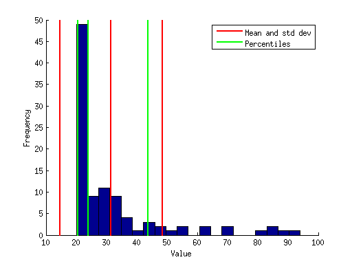
Example 1: Simple data plotting
% generate some fake data
x = (randn(1,100).^2)*10 + 20;

% compute some simple data summary metrics
mn = mean(x);  % compute mean
sd = std(x);   % compute standard deviation
ptiles = prctile(x,[16 50 84]);  % compute percentiles (median and central 68%)

% make a figure
figure;
hold on;
hist(x,20);  % plot a histogram using twenty bins
ax = axis;   % get the current axis bounds
  % plot lines showing mean and +/- 1 std dev
h1 = plot([mn mn],      ax(3:4),'r-','LineWidth',2);
h2 = plot([mn-sd mn-sd],ax(3:4),'r-','LineWidth',2);
h3 = plot([mn+sd mn+sd],ax(3:4),'r-','LineWidth',2);
  % plot lines showing percentiles
h4 = [];
for p=1:length(ptiles)
  h4(p) = plot(repmat(ptiles(p),[1 2]),ax(3:4),'g-','LineWidth',2);
end
legend([h1 h4(1)],{'Mean and std dev' 'Percentiles'});
xlabel('Value');
ylabel('Frequency');
Example 2: Monte Carlo simulations of correlation values
% define
numsim = 10000;   % number of simulations to run
samplesize = 50;  % number of data points in each sample

% pre-allocate the results vector
results = zeros(1,numsim);

% loop over simulations
for num=1:numsim

  % draw two sets of random numbers, each from the normal distribution
  data = randn(samplesize,2);

  % compute the correlation between the two sets of numbers and store the result
  results(num) = corr(data(:,1),data(:,2));

end

% visualize the results
figure; hold on;
hist(results,100);
ax = axis;
mx = max(abs(ax(1:2)));  % make the x-axis symmetric around 0
axis([-mx mx ax(3:4)]);
xlabel('Correlation value');
ylabel('Frequency');
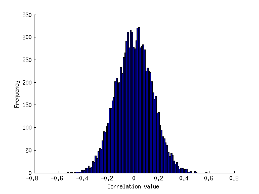
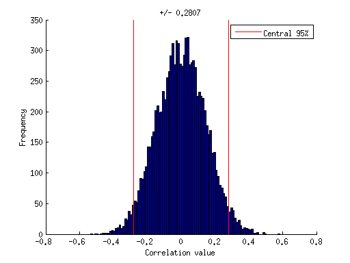
% although the two sets of numbers were drawn from independent
% probability distributions (and so should on average exhibit
% zero correlation), due to our limited sample size, we sometimes
% observe positive or negative correlation values.  what is the
% value below which most correlation magnitudes lie?  let's use
% 95% as the definition of "most".
val = prctile(abs(results),95);
val
val =

         0.280698330593468
% visualize this on the figure
ax = axis;
h1 = plot([val val],ax(3:4),'r-');
h2 = plot(-[val val],ax(3:4),'r-');
legend(h1,'Central 95%');
title(sprintf('+/- %.4f',val));
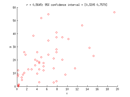
Example 3: Use bootstrapping to obtain confidence intervals on a correlation
% generate some fake data
x = [2.5 2.8 3.4 2 1.2 2.1 1.8 2.8 1.1 2.2 3.2 0.61 3 0.53 2 0.45 2 ...
     1 -0.53 1.2 2.2 2.5 1.9 1.9 2.8 2.8 1.3 3.1 2.7 2.3 0.47 2.1 1.5 3.8 ...
     3 2.8 0.97 2.5 2.3 3.9 0.54 3.6 2.3 2.7 4.4 2.7 0.44 2.1 1.7 2.1].^2;
y = [5.9 6.4 3.7 3.1 5.1 3.6 6.2 5.1 3 4.7 6 1.2 6.1 -0.51 4.4 3 ...
     5.1 2.2 0.14 3.2 7.2 7.4 4 4.5 5.3 2 4.9 3 4.6 3.9 3.5 4.2 3.6 5.4 ...
     4.5 6.1 2.6 4.9 3.5 4.8 1 6.8 4.2 3.7 7.5 1.7 2.8 1.8 3.6 4.3].^2;

% compute the actual correlation value observed
actualcorr = corr(x(:),y(:));

% draw bootstrap samples and compute correlation values
results = zeros(1,10000);
for num=1:10000

  % vector of indices (each element is a random integer between
  % 1 and n where n is the number of data points)
  ix = ceil(length(x) * rand(1,length(x)));

  % compute correlation using those data points
  results(num) = corr(x(ix)',y(ix)');

end

% alternatively, you could use MATLAB's bootstrp.m function to achieve the same result:
%   results = bootstrp(10000,@(x0,y0) corr(x0,y0),x',y');

% what is the central 95% of the bootstrap results?
ptiles = prctile(results,[2.5 97.5]);

% visualize
figure; hold on;
scatter(x,y,'ro');
xlabel('x');
ylabel('y');
title(sprintf('r = %.4f; 95%% confidence interval = [%.4f %.4f]',actualcorr,ptiles(1),ptiles(2)));
Example 4: Use randomization to assess the statistical significance of a correlation
% generate some fake data
x = [0.84 0.29 0.84 0.85 0.021 0.52 1 0.64 0.27 0.55 0.078 0.26 0.78 0.67 0.37 0.22 0.62 0.39 0.71 0.24];
y = [0.52 0.38 0.21 0.27 0.83 0.65 0.64 0.26 0.34 0.55 0.87 0.21 0.22 0.84 0.42 0.23 0.68 0.68 0.64 0.61];

% compute the actual correlation value observed
actualcorr = corr(x(:),y(:));

% we pose the null hypothesis that there is no dependency between the
% x-values and the y-values.  thus, under the null hypothesis, we should
% be able to break the association between x and y.

% perform randomization
results = zeros(1,10000);
for num=1:10000

  % vector of indices (a random ordering of the integers between
  % 1 and n where n is the number of data points)
  ix = randperm(length(x));

  % compute correlation between randomly shuffled x-values and the y-values
  results(num) = corr(x(ix)',y');

end

% visualize
figure; hold on;
hist(results,100);
ax = axis;
plot(repmat(actualcorr,[1 2]),ax(3:4),'r-');
  % compute the p-value as the fraction of the distribution that
  % is more extreme than the actually observed correlation value.
  % we use absolute value so that both positive and negative correlations
  % count as "extreme".  this is referred to as a two-tailed test.
pval = sum(abs(results) > abs(actualcorr)) / length(results);
title(sprintf('r = %.4f; p-value (two-tailed) = %.6f',actualcorr,pval));
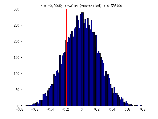
% the actual correlation value (-0.2) is fairly weak.  under the null
% hypothesis, we would expect to find correlation values of that size
% or larger about 40% of the time.  thus, we do not have sufficient
% evidence to reject the null hypothesis.  in other words, the
% actual correlation value observed is deemed not statistically
% significant.