MATLAB Examples 2 (covering Statistics Lectures 3 and 4)
Contents
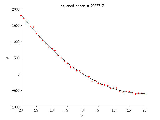
Example 1: Fit a linearized regression model
% generate some random data
x = -20:20;
y = 1.5*x.^2 - 60*x + 10 + 30*randn(size(x));

% given these data, we will now try to fit a model
% to the data.  we assume we know what model to use,
% namely, y = ax^2 + bx + c where a, b, and c are
% free parameters.  notice that this was the model
% we used to generate the data.

% since our model is a linearized model, we can express
% it using simple matrix notation.

% construct the regressor matrix
X = [x(:).^2 x(:) ones(length(x),1)];

% estimate the free parameters of the model
% using ordinary least-squares (OLS) estimation
w = inv(X'*X)*X'*y(:);

% what are the estimated weights?
w
w =

           1.5368275257135
          -60.638944801903
          8.15661270608602
% what is the model fit?
modelfit = X*w;

% what is the squared error achieved by this model fit?
squarederror = sum((y(:)-modelfit).^2);

% visualize
figure;
hold on;
scatter(x,y,'r.');
ax = axis;
xx = linspace(ax(1),ax(2),100)';
yy = [xx.^2 xx ones(length(xx),1)]*w;
plot(xx,yy,'k-');
xlabel('x');
ylabel('y');
title(sprintf('squared error = %.1f',squarederror));
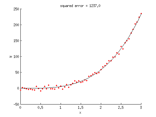
Example 2: Fit a parametric nonlinear model
% generate some random data
x = 0:.05:3;
y = 5*x.^3.5 + 5*randn(size(x));

% given these data, we will now try to fit a model
% to the data.  we assume we know what model to use,
% namely, y = ax^n where a and n are free parameters.
% notice that this was the model we used to generate the data.

% define optimization options
options = optimset('Display','iter','FunValCheck','on', ...
                   'MaxFunEvals',Inf,'MaxIter',Inf, ...
                   'TolFun',1e-6,'TolX',1e-6);

% define bounds for the parameters
%              a    n
paramslb = [-Inf    0];  % lower bound
paramsub = [ Inf  Inf];  % upper bound

% define the initial seed
%            a     n
params0 = [  1     1];

% estimate the free parameters of the model using nonlinear optimization
  % hint: pp is a vector of parameters like [a n],
  %       xx is a vector of x-values like [.1 .4 .5],
  %       and what modelfun does is to output the predicted y-values.
modelfun = @(pp,xx) pp(1)*xx.^pp(2);
[params,resnorm,residual,exitflag,output] = lsqcurvefit(modelfun,params0,x,y,paramslb,paramsub,options);
                                         Norm of      First-order
 Iteration  Func-count     f(x)          step          optimality   CG-iterations
     0          3          431921                      7.93e+03
     1          6          431921             10       7.93e+03            0
     2          9          247013            2.5        8.3e+04            0
     3         12          247013        2.81299        8.3e+04            0
     4         15         98286.2       0.703246       1.09e+05            0
     5         18         17315.7        1.40649       3.78e+05            0
     6         21         1894.05       0.327179       2.46e+04            0
     7         24         1482.46       0.939262       9.09e+03            0
     8         27         1241.08       0.422605       1.33e+03            0
     9         30         1237.01     0.00758631            5.5            0
    10         33         1237.01    1.29563e-05       7.82e-05            0

Local minimum possible.

lsqcurvefit stopped because the final change in the sum of squares relative to
its initial value is less than the selected value of the function tolerance.
% what are the estimated parameters?
params
params =

           5.4338041940236          3.42528833322854
% what is the model fit?
modelfit = modelfun(params,x);

% what is the squared error achieved by this model fit?
squarederror = sum((y(:)-modelfit(:)).^2);
% (note that the 'resnorm' output also provides the squared error.)

% visualize
figure;
hold on;
scatter(x,y,'r.');
ax = axis;
xx = linspace(ax(1),ax(2),100)';
yy = modelfun(params,xx);
plot(xx,yy,'k-');
xlabel('x');
ylabel('y');
title(sprintf('squared error = %.1f',squarederror));
Example 3: Another optimization example
% generate some random data
x = rand(1,1000).^2;

% we want to determine the value that minimizes the sum of the
% absolute differences between the value and the data points

% define some stuff
options = optimset('Display','iter','FunValCheck','on', ...
                   'MaxFunEvals',Inf,'MaxIter',Inf, ...
                   'TolFun',1e-6,'TolX',1e-6);
paramslb = [];  % [] means no bounds
paramsub = [];
params0 = [0];

% perform the optimization
  % hint: here we have to apply a square-root transformation so that when
  % lsqnonlin squares the output of costfun, we will be back to absolute error.
costfun = @(pp) sqrt(abs(x-pp));
[params,resnorm,residual,exitflag,output] = lsqnonlin(costfun,params0,paramslb,paramsub,options);
                                         Norm of      First-order
 Iteration  Func-count     f(x)          step          optimality   CG-iterations
     0          2          346.47                           500
     1          4         346.385    8.61928e-05            490            0
     2          6         341.862     0.00491093            440            0
     3          8         333.538      0.0101418            387            0
     4         10         315.811      0.0259447            306            0
     5         12         308.364      0.0129775            271            0
     6         14         292.776      0.0324211            215            0
     7         16          279.22       0.035143            170            0
     8         18          270.08      0.0314543            118            0
     9         20         263.724       0.031138             88            0
    10         22         259.555      0.0265819             67            0
    11         24         258.266      0.0107348             52            0
    12         26         257.181       0.012298             35            0
    13         28         256.649     0.00864949             25            0
    14         30         256.518     0.00310659             19            0
    15         32         256.401     0.00335775             15            0
    16         34         256.317     0.00312291             12            0
    17         36         256.252     0.00307883              7            0
    18         38         256.245    0.000546973              6            0
    19         40         256.236    0.000864426              5            0
    20         42         256.227      0.0010377              4            0
    21         44         256.224    0.000510969              3            0
    22         46          256.22    0.000677599              3            0
    23         48         256.218    0.000404828              1            0
    24         50         256.218    0.000140253              1            0
    25         52         256.217    0.000193302              1            0
    26         54         256.217     0.00021431              1            0
    27         56         256.217    0.000205629              1            0
    28         58         256.216    9.93736e-05       5.88e-05            0

Local minimum possible.

lsqnonlin stopped because the final change in the sum of squares relative to
its initial value is less than the selected value of the function tolerance.
% what is the solution?
params
params =

         0.260043242623885
% what is the median of the data?
median(x)
ans =

         0.260365029783367
% notice that the solution is nearly identical to the median of the data.
% (the slop comes from the tolerance used in the optimization and
% from the interpolation used in the calculation of the median.)