MATLAB Examples 3 (covering Statistics Lectures 5 and 6)

Contents

Example 1: Demonstration of various types of resampling

% define a set of data
data = randn(1,100);  % 100 data points
n = length(data);     % the number of data points

% in bootstrapping, we draw n points with replacement from a
% set of n data points.
numboots = 1000;               % how many bootstraps to perform
for p=1:numboots
  bootix = ceil(n*rand(1,n));  % indices to use for the bootstrap sample
  % data(bootix) gives the bootstrap sample.
end

% in leave-one-out cross-validation, we leave out a data point,
% train on the remaining data points and then test on the left-out
% data point.  this process is repeated for each data point.
for p=1:n
  trainix = setdiff(1:n,p);  % indices to use for training
  testix = p;                % indices to use for testing
  % data(trainix) gives the training data
  % data(testix) gives the testing data
end

% in k-fold cross-validation, we divide the data into k parts,
% leave out one of the parts, train on the remaining parts,
% and then test on the left-out part.  this process is repeated
% for each part.
k = 8;                  % how many parts to use
allix = randperm(n);    % all data indices, randomly ordered
numineach = ceil(n/k);  % at least one part must have this many data points
  % add NaNs and reshape data indices into a 2D matrix.
  % this process ensures that the numbers of data points in each part
  % are as evenly balanced as possible.
allix = reshape([allix NaN(1,k*numineach-n)],k,numineach);
for p=1:k
  testix = allix(p,:);            % indices to use for testing
  testix(isnan(testix)) = [];     % remove NaNs if necessary
  trainix = setdiff(1:n,testix);  % indices to use for training
  % data(trainix) gives the training data
  % data(testix) gives the testing data
end

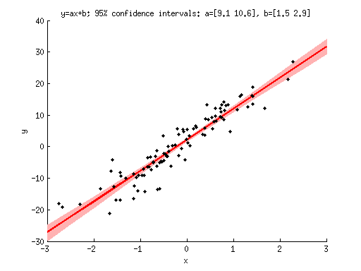
Example 2: Bootstrap a simple linear model

% generate some data
n = 100;
x = randn(1,n);
y = 10*x + 2 + 4*randn(1,n);

% define
numboots = 10000;  % number of bootstraps to perform
xvals = -3:.5:3;   % x-values to evaluate the model at

% perform the bootstraps
modelfit = zeros(numboots,length(xvals));
params = zeros(numboots,2);
for boot=1:numboots

  % prepare data indices
  ix = ceil(n*rand(1,n));

  % construct regressor matrix
  X = [x(ix)' ones(n,1)];

  % estimate parameters
  h = inv(X'*X)*X'*y(ix)';

  % evaluate the model
  modelfit(boot,:) = xvals*h(1) + h(2);

  % record the parameters
  params(boot,:) = h;

end

% visualize
figure;
hold on;
h1 = scatter(x,y,'k.');
modelfitP = prctile(modelfit,[2.5 50 97.5],1);
  % define a polygon by following the 2.5th percentile line (left to right)
  % and then reversing and following the 97.5th percentile line (right to left).
h2 = patch([xvals fliplr(xvals)],[modelfitP(1,:) fliplr(modelfitP(3,:))],[1 .7 .7]);
set(h2,'EdgeColor','none');
h3 = plot(xvals,modelfitP(2,:),'r-','LineWidth',2);
uistack(h1,'top');  % make sure data points are visible by bringing them to the top
xlabel('x');
ylabel('y');
paramsP = prctile(params,[2.5 97.5],1);
title(sprintf('y=ax+b; 95%% confidence intervals: a=[%.1f %.1f], b=[%.1f %.1f]', ...
              paramsP(1,1),paramsP(2,1),paramsP(1,2),paramsP(2,2)));

Example 3: Perform leave-one-out cross-validation for a simple linear model

% reuse data from previous example
n = n;
x = x;
y = y;

% perfom leave-one-out cross-validation
predictions = zeros(1,n);  % this will hold the prediction for each data point
for p=1:n

  % figure out indices
  trainix = setdiff(1:n,p);
  testix = p;

  % train the model
  X = [x(trainix)' ones(length(trainix),1)];  % construct regressor matrix
  h = inv(X'*X)*X'*y(trainix)';               % estimate parameters

  % test the model by computing the prediction for the left-out data point
  predictions(p) = [x(testix)' ones(length(testix),1)]*h;

end

% quantify how well the predictions match the data using coefficient of determination
R2 = 100 * (1 - sum((y-predictions).^2) / sum((y-mean(y)).^2));

% report the answer
fprintf('Cross-validated R^2 = %.2f%%\n',R2);

Cross-validated R^2 = 87.89%

Published with MATLAB® R2012b