MATLAB Examples 4 (covering Statistics Lecture 7)

Contents

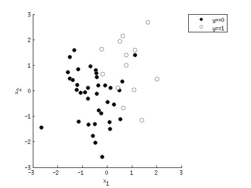
Example 1: Simple 2D classification using logistic regression

% generate some data (50 data points defined in two dimensions;
% class assignment is 0 or 1 for each data point)
x1 = randn(50,1);
x2 = randn(50,1);
y = (2*x1 + x2 + randn(size(x1))) > 1;

% visualize the data
figure; hold on;
h1 = scatter(x1(y==0),x2(y==0),50,'k','filled');  % black dots for 0
h2 = scatter(x1(y==1),x2(y==1),50,'w','filled');  % white dots for 1
set([h1 h2],'MarkerEdgeColor',[.5 .5 .5]);        % outline dots in gray
legend([h1 h2],{'y==0' 'y==1'},'Location','NorthEastOutside');
xlabel('x_1');
ylabel('x_2');

% define optimization options
options = optimset('Display','iter','FunValCheck','on', ...
                   'MaxFunEvals',Inf,'MaxIter',Inf, ...
                   'TolFun',1e-6,'TolX',1e-6);

% define logistic function (this takes a matrix of values and
% applies the logistic function to each value)
logisticfun = @(x) 1./(1+exp(-x));

% construct regressor matrix
X = [x1 x2];
X(:,end+1) = 1;  % we need to add a constant regressor

% define initial seed
params0 = zeros(1,size(X,2));

% define bounds
paramslb = [];  % [] means no bounds
paramsub = [];

% define cost function (negative-log-likelihood)
  % here, the eps is a hack to ensure that the log returns a finite number.
costfun = @(pp) -sum((y .* log(logisticfun(X*pp')+eps)) + ...
                     ((1-y) .* log(1-logisticfun(X*pp')+eps)));

% fit the logistic regression model by finding
% parameter values that minimize the cost function
[params,resnorm,residual,exitflag,output] = ...
  lsqnonlin(costfun,params0,paramslb,paramsub,options);

Warning: Trust-region-reflective algorithm requires at least as many equations
as variables; using Levenberg-Marquardt algorithm instead. 

                                        First-Order                    Norm of 
 Iteration  Func-count    Residual       optimality      Lambda           step
     0           4         1201.13             544         0.01
     1           8         249.865            66.7        0.001        1.57413
     2          12         162.838            16.1       0.0001        3.09029
     3          22         157.936            10.8          100       0.168952
     4          26         155.321             7.6           10       0.120881
     5          30         153.054            14.6            1        0.91166
     6          36         148.397            7.02          100       0.173822
     7          40         147.149            3.24           10       0.090581
     8          45         146.815            1.57          100       0.046862
     9          49         146.718            1.02           10      0.0248996
    10          54         146.682           0.807          100        0.01455
    11          58         146.665           0.669           10     0.00997112
    12          62         146.643           0.809            1      0.0786498
    13          68         146.624           0.377          100      0.0113596
    14          72         146.619           0.206           10     0.00539815
    15          77         146.618            0.12          100     0.00271585
    16          81         146.618          0.0742           10     0.00154244
    17          86         146.618           0.062          100     0.00104312
    18          90         146.617          0.0539           10    0.000814137

Local minimum possible.

lsqnonlin stopped because the final change in the sum of squares relative to 
its initial value is less than the selected value of the function tolerance.

% compute the output (class assignment) of the model for each data point
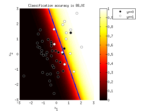
modelfit = logisticfun(X*params') >= 0.5;

% calculate percent correct (percentage of data points
% that are correctly classified by the model)
pctcorrect = sum(modelfit==y) / length(y) * 100;

% visualize the model
  % prepare a grid of points to evaluate the model at
ax = axis;
xvals = linspace(ax(1),ax(2),100);
yvals = linspace(ax(3),ax(4),100);
[xx,yy] = meshgrid(xvals,yvals);
  % construct regressor matrix
X = [xx(:) yy(:)];
X(:,end+1) = 1;
  % evaluate model at the points (but don't perform the final thresholding)
outputimage = reshape(logisticfun(X*params'),[length(yvals) length(xvals)]);
  % visualize the image (the default coordinate system for images
  % is 1:N where N is the number of pixels along each dimension.
  % we have to move the image to the proper position; we
  % accomplish this by setting XData and YData.)
h3 = imagesc(outputimage,[0 1]);  % the range of the logistic function is 0 to 1
set(h3,'XData',xvals,'YData',yvals);
colormap(hot);
colorbar;
  % visualize the decision boundary associated with the model
  % by computing the 0.5-contour of the image
[c4,h4] = contour(xvals,yvals,outputimage,[.5 .5]);
set(h4,'LineWidth',3,'LineColor',[0 0 1]);  % make the line thick and blue
  % send the image to the bottom so that we can see the data points
uistack(h3,'bottom');
  % send the contour to the top
uistack(h4,'top');
  % restore the original axis range
axis(ax);
  % report the accuracy of the model in the title
title(sprintf('Classification accuracy is %.1f%%',pctcorrect));

% try a 3D visualization
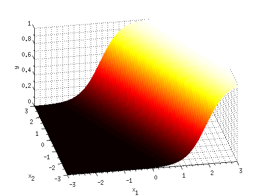
figure; hold on;
h1 = surf(xvals,yvals,outputimage);
set(h1,'EdgeAlpha',0);  % don't show the edges of the surface
colormap(hot);
xlabel('x_1');
ylabel('x_2');
zlabel('y');
view(-11,42);  % set the viewing angle
  % show some grid lines for reference
set(gca,'XGrid','on','XMinorGrid','on', ...
        'YGrid','on','YMinorGrid','on', ...
        'ZGrid','on','ZMinorGrid','on');

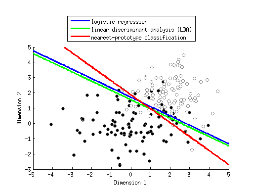
Example 2: Compare solutions of different classifiers

% generate some data (two classes of data points defined in two dimensions)
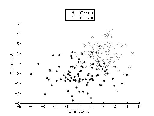
classA = bsxfun(@times,[1.5 1]',randn(2,100));
classB = 2+randn(2,100);

% visualize the data
figure; hold on;
h1 = scatter(classA(1,:),classA(2,:),'ko','filled');
h2 = scatter(classB(1,:),classB(2,:),'wo','filled');
set([h1 h2],'MarkerEdgeColor',[.5 .5 .5]);
legend([h1 h2],{'Class A' 'Class B'},'Location','NorthOutside');
xlabel('Dimension 1');
ylabel('Dimension 2');

% prepare a grid of points to evaluate the model at
ax = axis;
xvals = linspace(ax(1),ax(2),200);
yvals = linspace(ax(3),ax(4),200);
[xx,yy] = meshgrid(xvals,yvals);
gridX = [xx(:) yy(:)];

% perform logistic regression (here we use the MATLAB function glmfit.m
% instead of the direct implementation shown in Example 1)
X = [classA(1,:)' classA(2,:)';
     classB(1,:)' classB(2,:)'];
y = [zeros(size(classA,2),1); ones(size(classB,2),1)];
paramsA = glmfit(X,y,'binomial','link','logit');
outputimageA = glmval(paramsA,gridX,'logit');
outputimageA = reshape(outputimageA,[length(yvals) length(xvals)]);
[d,hA] = contour(xvals,yvals,outputimageA,[.5 .5]);
set(hA,'LineWidth',3,'LineColor',[0 0 1]);  % make the line thick and blue

% perform linear discriminant analysis (here we use the MATLAB function
% classify.m; ideally, we would implement it from scratch so we really
% understand how it works!)
outputimageB = classify(gridX,X,y,'linear');
outputimageB = reshape(outputimageB,[length(yvals) length(xvals)]);
[d,hB] = contour(xvals,yvals,outputimageB,[.5 .5]);
set(hB,'LineWidth',3,'LineColor',[0 1 0]);  % make the line thick and green

% nearest-prototype classification
centroidA = mean(classA,2);  % 2 x 1
centroidB = mean(classB,2);  % 2 x 1
  % compute distance to centroid A
disttoA = sqrt(sum(bsxfun(@minus,gridX,centroidA').^2,2));
  % compute distance to centroid B
disttoB = sqrt(sum(bsxfun(@minus,gridX,centroidB').^2,2));
outputimageC = disttoA > disttoB;
outputimageC = reshape(outputimageC,[length(yvals) length(xvals)]);
[d,hC] = contour(xvals,yvals,outputimageC,[.5 .5]);
set(hC,'LineWidth',3,'LineColor',[1 0 0]);  % make the line thick and red

% add legend
legend([hA hB hC],{'logistic regression' ...
                   'linear discriminant analysis (LDA)' ...
                   'nearest-prototype classification'}, ...
       'Location','NorthOutside');

Published with MATLAB® R2012b