FID Load Option

 

  
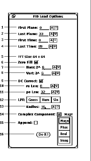
Figure 8: FID format options popup window

  
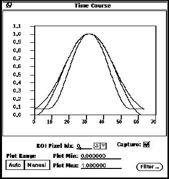
Figure 9: LPF 1D filter profiles

For loading an image set with fid format[6], the options are shown in Figure 8. The fid can only have a single phase encode and must have the slcto or pss parameter set. The following is a list of steps for specifying options for the loading of an image with fid format:

1. The first step in loading a fid image is to specify the spatial and temporal parameters. When the popup window comes up, the First Plane (8-1) and Last Plane (8-2) fields are set to the indices that yield the full spatial extent of the image volume. Thus the first plane is set to 0 and the last plane is set to the number of planes minus one. For stim files the temporal range is specified by the First Time (8-3) and Last Time (8-4) fields, and by default are set to yield the full temporal range. A subset of the data can be specified by modifying the planar and temporal range. As anat files are only 3D spatially, the last time field is not displayed, but the first time can be used to select a particular volume out of a 4D data set.
2. As fids require FFT processing, there are several processing options available. When the Zero Fill option (8-6) is selected, the fid can be buffered to any size that is a power of two in either or both of the Horiz (8-7) or Vert (8-8) planar dimension. The FFT Size (8-5) field displays the planar buffer size as it is modified.
3. When there is a DC offset in the fid data, the post-FFT image will exhibit a bright spot in the center of the image. Since the fid decays to zero at the borders of the image, an effective correction method is to take an average of the fid tails and subtract this average from the entire pre-FFT image. By selecting the DC Correct option (8-9), the number of complex points along the read out direction (ro Len 8-10) and the phase encode (pe Len 8-11) direction for the tail average can be specified. An average complex value is calculated from points in each corner. Thus the average from these (4 x pe Len x ro Len) points is subtracted from every point in each planar image prior to the FFT.
4. If it is desired to reduce high frequency 2D spatial noise, a LPF (Low Passs Filter) can be used by selecting a LPF choice (8-12). Then prior to the FFT, the fid image is multiplied by the specified 2D filter. Examples of the LPF profiles are shown in Figure 9.

   The gaussian filter has a FWHM (Full Width - Half Maximum) equal to twice the radius specified in Radius field (8-13). The values, g(n), of the gaussian filter are given for one dimension in Equation 1 for a radius = r and an image width of N pixels.

   
    
   

   The values, s(n), of the sinusoidal filter are given for one dimension in Equation 2 for a radius = r (8-13) and an image width of N pixels.

   
    
   

   The values, h(n), of the hamming filter are given for one dimension in Equation 3 for a radius = r (8-13) and an image width of N pixels.

   
    
   

5. Normally the magnitude of the complex FFT result is desired. However, under certain experimental situations it may be desirable to use another complex component. The menu under the Complex Component button (8-14) allows the option of magnitude, phase, real or imaginary to be chosen.
6. When loading stim image files, the Append (8-15) option is available. When this option is selected, the image volume(s) specified for loading are appended across time to the currently loaded stimulation set of image volumes. Note that the new image volumes to be appended must have the same spatial dimensions as those currently loaded.
7. Lastly, when all the options are set, press the Do It button (8-16) to invoke the loading process. See Section 7 for the procedure to display the images.